RSF Direction Ionogram and Daily Directogram
Echo Direction Visualization — Figure 3-8 and Figure 3-12 Style
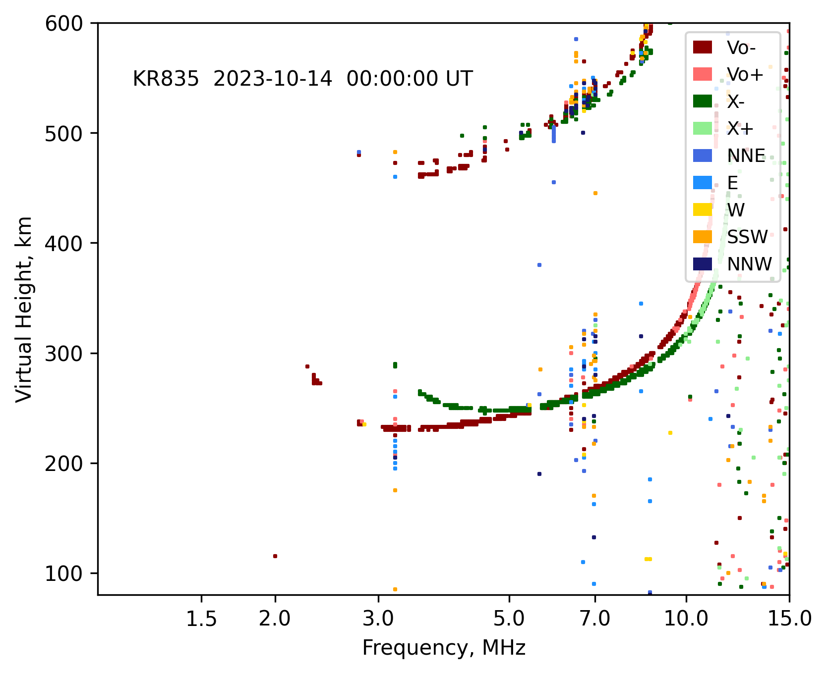
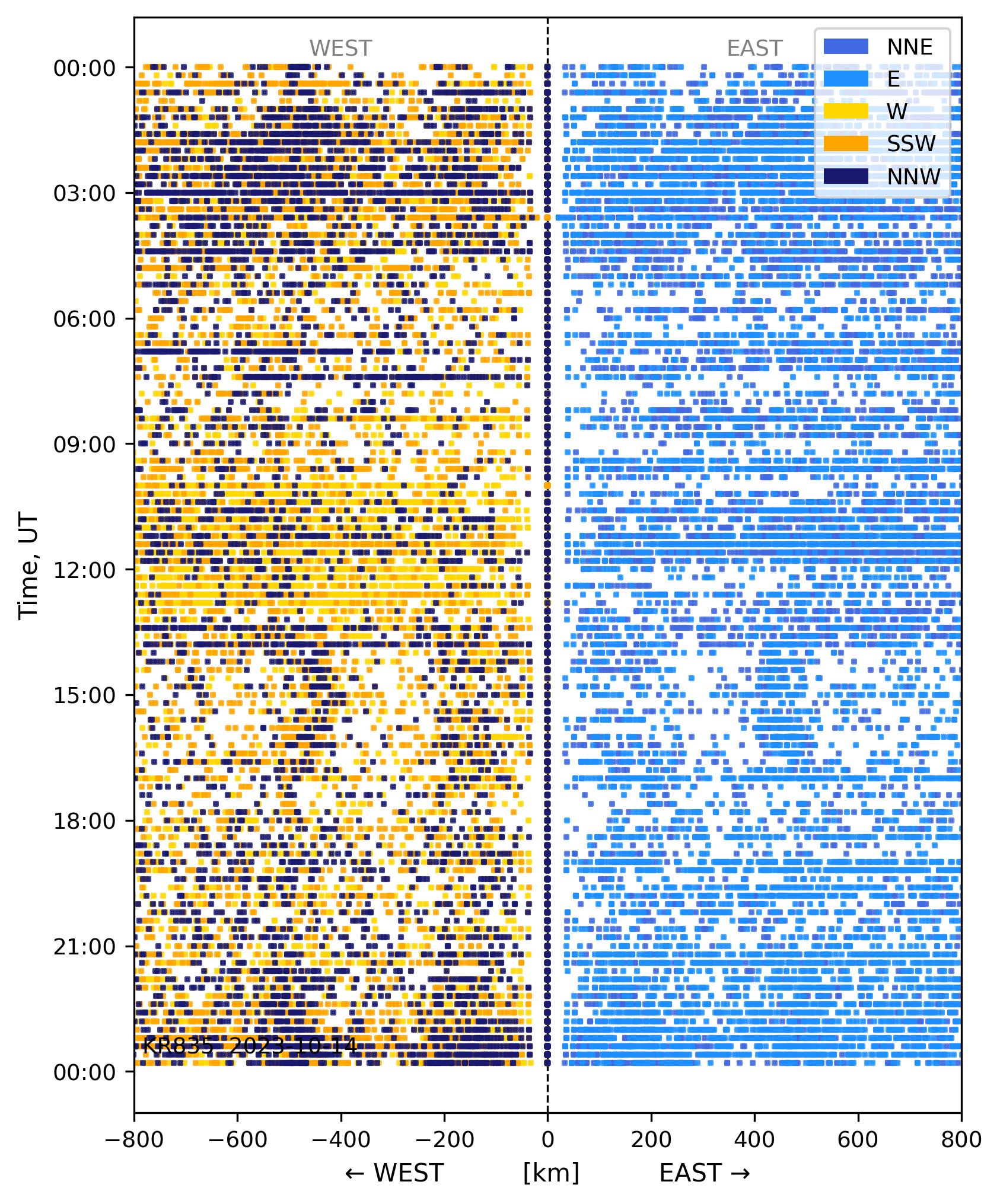
Produce a direction-coded ionogram for a single RSF sounding (mimicking Digisonde-4D Manual Figure 3-8) and a full-day directogram stacking all soundings by UT time with West–East ground distance on the x-axis (Figure 3-11/3-12 style).
This page explains examples/digisonde/rsf_direction_ionogram.py.
Data used: KR835 (Kirtland AFB), 14 October 2023, 480 RSF files.
Call Flow
Single direction-coded ionogram
RsfExtractor(filepath, ...)parses one.RSFfile..extract()→.to_pandas()flattens echoes to a DataFrame with columnsfrequency,height_km,amplitude,azimuth,doppler_num,polarization.RsfIonogram.add_direction_ionogram(...)classifies each echo into one of 10 direction+polarization categories (NoVal, NNE, E, W, Vo−, Vo+, SSW, X−, X+, NNW) and scatter-plots (log₁₀ frequency, height) with per-category colors matching Figure 3-8.- Legend uses
matplotlib.patches.Patchentries for each active category.
Daily directogram
glob.glob("KR835_*.RSF")collects all RSF files for the day.- A module-level
_load_rsfworker parses each file withRsfExtractor; failed files are skipped with a warning rather than aborting the run. multiprocessing.Pool.mapfans the worker across all files in parallel (N_PROCS = 8), then failed results (None) are filtered out beforepd.concat.RsfIonogram.add_directogram(...)groups echoes by ionogram timestamp, computes the vertical reference height H_v from peak vertical echoes, and derives ground distance D_i = √(H_i² − H_v²) with sign negative for westward arrivals.- Y-axis = UT time (
matplotlib.dates), X-axis = D_i (km), scatter colored by echo category.
Key Code
1) Single Ionogram — Direction-Coded
from pynasonde.digisonde.parsers.rsf import RsfExtractor
from pynasonde.digisonde.digi_plots import RsfIonogram

RSF_FILE = "path/to/KR835_2023287000000.RSF"

extractor = RsfExtractor(RSF_FILE, extract_time_from_name=True, extract_stn_from_name=True)
extractor.extract()
df = extractor.to_pandas()

h = extractor.rsf_data.rsf_data_units[0].header
title = f"KR835  {h.date.strftime('%Y-%m-%d  %H:%M:%S')} UT"

r = RsfIonogram(figsize=(6, 5), font_size=10)
r.add_direction_ionogram(
    df,
    ylim=[80, 600],
    xlim=[1, 15],
    xticks=[1.5, 2.0, 3.0, 5.0, 7.0, 10.0, 15.0],
    text=title,
    lower_plimit=5,
    ms=1.0,
)
r.save("docs/examples/figures/rsf_direction_ionogram_KR835.png")
r.close()
2) Daily Directogram — parallel loading
import glob

import pandas as pd
from joblib import Parallel, delayed
from loguru import logger
from pynasonde.digisonde.parsers.rsf import RsfExtractor
from pynasonde.digisonde.digi_plots import RsfIonogram

RSF_DIR = "path/to/SKYWAVE_DPS4D_2023_10_14"
N_PROCS = 8   # tune to available CPU cores


def _load_rsf(fpath: str) -> pd.DataFrame | None:
    """Parse one RSF file; return its DataFrame or None on failure."""
    try:
        ex = RsfExtractor(fpath, extract_time_from_name=True)
        ex.extract()
        return ex.to_pandas()
    except Exception as e:
        logger.warning(f"Skipped {fpath}: {e}")
        return None


all_files = sorted(glob.glob(f"{RSF_DIR}/KR835_*.RSF"))
logger.info(f"Loading {len(all_files)} RSF files with {N_PROCS} workers")

results = Parallel(n_jobs=N_PROCS, backend="loky")(
    delayed(_load_rsf)(fpath) for fpath in all_files
)

df_day = pd.concat(
    [df for df in results if df is not None],
    ignore_index=True,
)
logger.info(f"Total records: {len(df_day)}")

r = RsfIonogram(figsize=(6, 8), font_size=10)
r.add_directogram(
    df_day,
    dlim=[-800, 800],
    lower_plimit=5,
    ms=0.5,
    text="KR835  2023-10-14",
)
r.save("docs/examples/figures/rsf_directogram_KR835_daily.png")
r.close()
Why joblib instead of multiprocessing.Pool?
multiprocessing.Pool.map sends results back through an OS pipe whose
buffer is typically 64 KB. Large DataFrames overflow the pipe, causing
BrokenPipeError: [Errno 32]. joblib with the loky backend uses
memory-mapped temporary files for large objects, so arbitrarily large
DataFrames are returned safely. joblib is already a dependency of
pynasonde — no extra install needed.
Echo Direction Color Scheme
| Category | Color | Azimuth | Notes |
|---|---|---|---|
| NoVal | gray | — | Below amplitude threshold |
| NNE | royalblue | 0° | North / north-northeast |
| E | dodgerblue | 60° | East |
| W | gold | 120° | Southeast (maps west in D_i) |
| Vo− | darkred | vertical | Negative Doppler (downward layer) |
| Vo+ | lightcoral | vertical | Positive Doppler (upward layer) |
| SSW | orange | 180° | South / south-southwest |
| X− | darkgreen | — | X-mode, negative Doppler |
| X+ | lightgreen | — | X-mode, positive Doppler |
| NNW | midnightblue | 300° | North-northwest |
Ground Distance Formula
For each echo at virtual height H_i, ground distance is:
where H_v is the ionogram's vertical reference height (median of vertical echoes near the F-layer peak). Sign: negative for westward arrivals (SSW, NNW, W), positive for eastward (NNE, E).
Run
Output Figures
Related Files
examples/digisonde/rsf_direction_ionogram.pypynasonde/digisonde/parsers/rsf.pypynasonde/digisonde/digi_plots.py—RsfIonogram.add_direction_ionogram(),add_directogram()