SAO Isodensity Contours + DFT Doppler Waterfall and Spectra
Three-Figure Workflow: Isodensity, Waterfall, and Spectra
Build a daily isodensity contour from 240 SAO files, then visualize the Doppler waterfall and per-height spectra from a single DFT drift file — all three plots in one script.
This page explains examples/digisonde/sao_iso_dft_plots.py.
Data used: KR835 (Kirtland AFB), 14 October 2023 —
240 .SAO files + KR835_2023287000915.DFT.
Call Flow
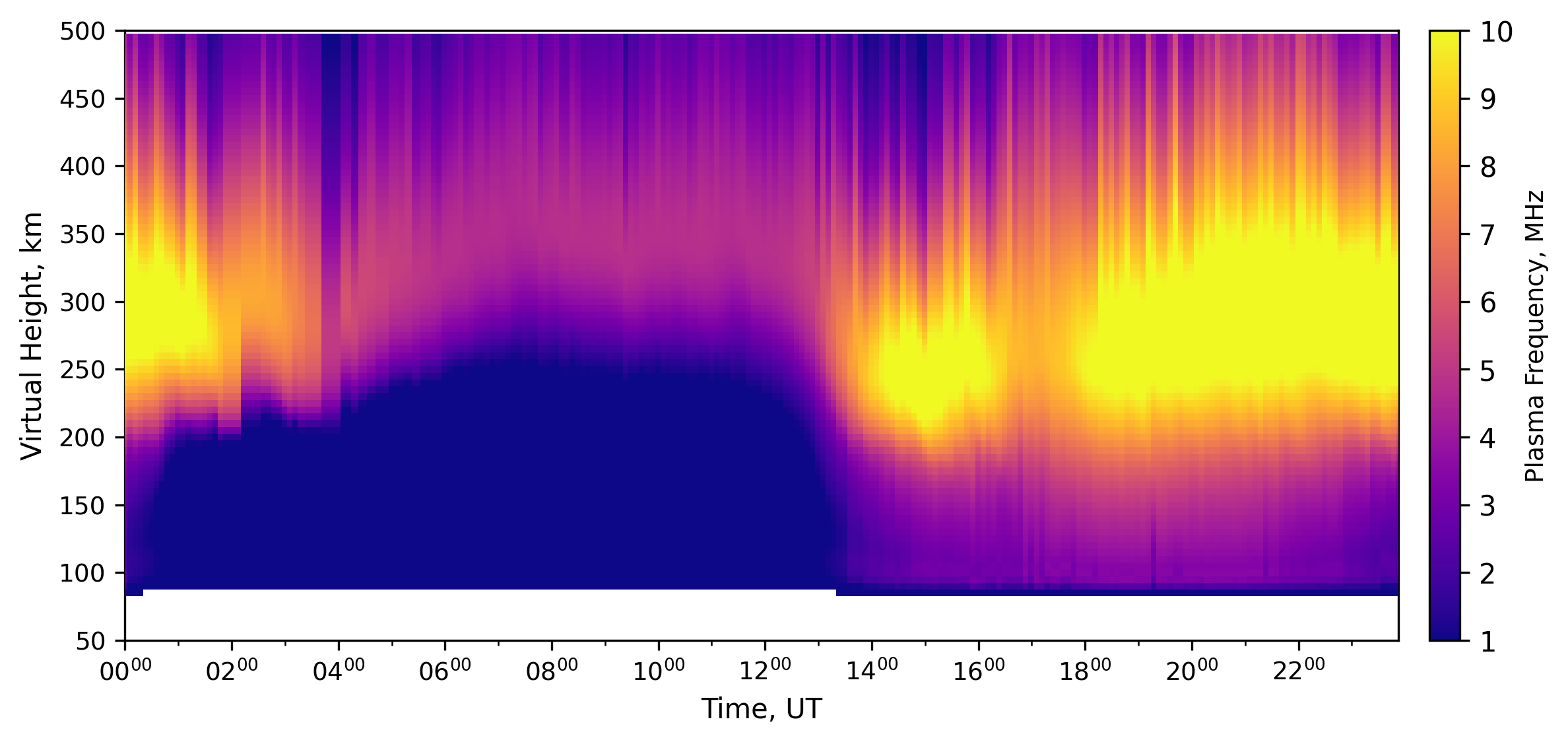
Figure 1 — Isodensity contour
SaoExtractor.load_SAO_files(...)loads all 240 SAO files in parallel.df["datetime"]is cast topd.Timestampfor the time axis.SaoSummaryPlots.add_isodensity_contours(...)bins height to a 5 km grid withpd.cut+groupby, renders apcolormeshcolored by mean plasma frequency, and overlayscontourlines at each integer MHz level (mimicking Digisonde-Isodensity.gif).
Figure 2 — Doppler waterfall
DftExtractor(filepath, ...)opens the DFT file and counts blocks..extract()iterates all 96 blocks, unpacking 16 sub-cases × 128 amplitude bytes + 128 phase bytes per sub-case. Header bits are decoded from the LSBs of all amplitude bytes..to_pandas()flattens to rows of(block_idx, subcase_idx, height_km, doppler_bin, amplitude, phase, frequency_hz, date).SkySummaryPlots.plot_doppler_waterfall(...)auto-selects the block with peak amplitude, computes the 2nd–98th percentile color range, and renders apcolormeshof Doppler bin vs. height.
Figure 3 — Doppler spectra
- Same DataFrame from step 3 above.
SkySummaryPlots.plot_doppler_spectra(...)auto-selects the same best block, samplesn_heightsevenly-spaced height bins, and plots one amplitude-vs-Doppler line per height, colored by viridis.
Key Code
1) SAO Isodensity Contours
import pandas as pd
from pynasonde.digisonde.parsers.sao import SaoExtractor
from pynasonde.digisonde.digi_plots import SaoSummaryPlots

SAO_DIR = "path/to/SKYWAVE_DPS4D_2023_10_14"

df_sao = SaoExtractor.load_SAO_files(
    folders=[SAO_DIR],
    ext="KR835_*.SAO",
    n_procs=8,
    func_name="height_profile",
)
df_sao = df_sao.reset_index(drop=True)
df_sao["datetime"] = pd.to_datetime(df_sao["datetime"])

p = SaoSummaryPlots(figsize=(10, 4), font_size=10)
p.add_isodensity_contours(
    df_sao,
    xparam="datetime",
    yparam="th",
    zparam="pf",
    ylim=[50, 500],
    fbins=[1, 2, 3, 4, 5, 6, 7, 8, 9, 10],
    text="KR835  2023-10-14",
)
p.save("docs/examples/figures/sao_isodensity_KR835.png")
p.close()
2) DFT Doppler Waterfall
from pynasonde.digisonde.parsers.dft import DftExtractor
from pynasonde.digisonde.digi_plots import SkySummaryPlots

DFT_FILE = f"{SAO_DIR}/KR835_2023287000915.DFT"

dft = DftExtractor(DFT_FILE, extract_time_from_name=True, extract_stn_from_name=True)
dft.extract()
df_dft = dft.to_pandas()
title_dft = f"KR835  {dft.date.strftime('%Y-%m-%d  %H:%M:%S')} UT"

sk = SkySummaryPlots(figsize=(7, 5), font_size=10, subplot_kw={})
sk.plot_doppler_waterfall(
    df_dft,
    cmap="inferno",
    text=title_dft,
)
sk.save("docs/examples/figures/dft_doppler_waterfall_KR835.png")
sk.close()
3) DFT Doppler Spectra
sk2 = SkySummaryPlots(figsize=(7, 4), font_size=10, subplot_kw={})
sk2.plot_doppler_spectra(
    df_dft,
    n_heights=8,
    cmap="viridis",
    text=title_dft,
)
sk2.save("docs/examples/figures/dft_doppler_spectra_KR835.png")
sk2.close()
subplot_kw override
SkySummaryPlots defaults to a polar projection for skymap use.
Always pass subplot_kw={} when creating waterfall or spectra plots.
DFT Height Decoding
Virtual height is estimated from the block header fields:
where height_resolution is the raw 4-bit header value (typical value = 2,
giving 10 km steps). For the KR835 file this yields heights 100–250 km —
physically reasonable for E/F-layer sounding at ~6.5 MHz.
Run
Output Figures
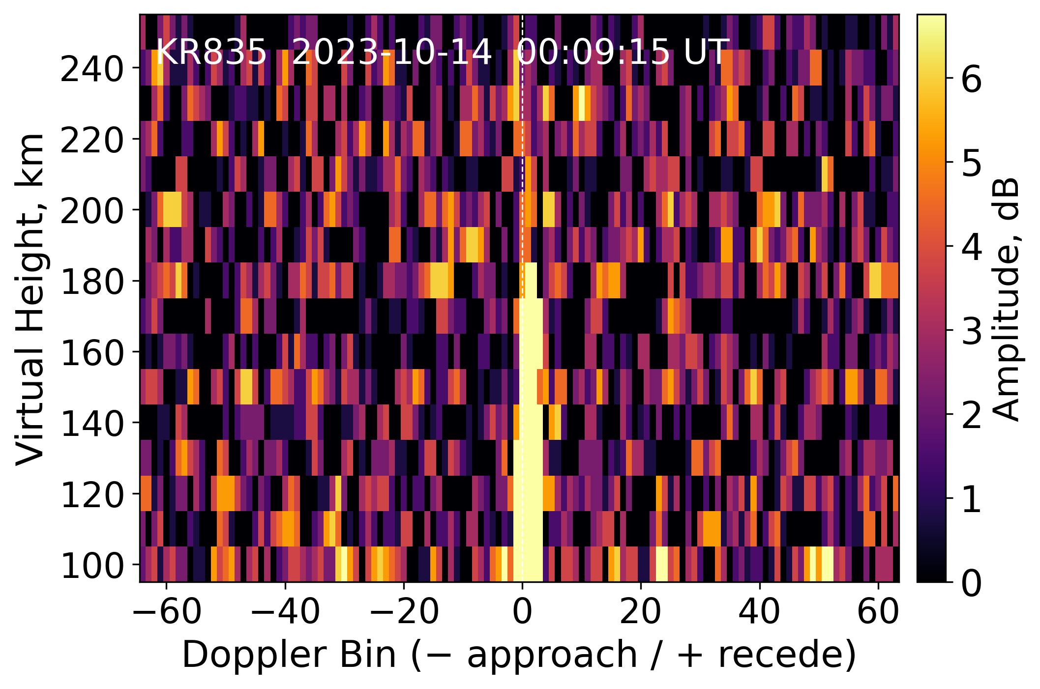
KR835_2023287000915.DFT. Doppler bin on the x-axis, height on the y-axis; amplitude color highlights the dominant drift signal.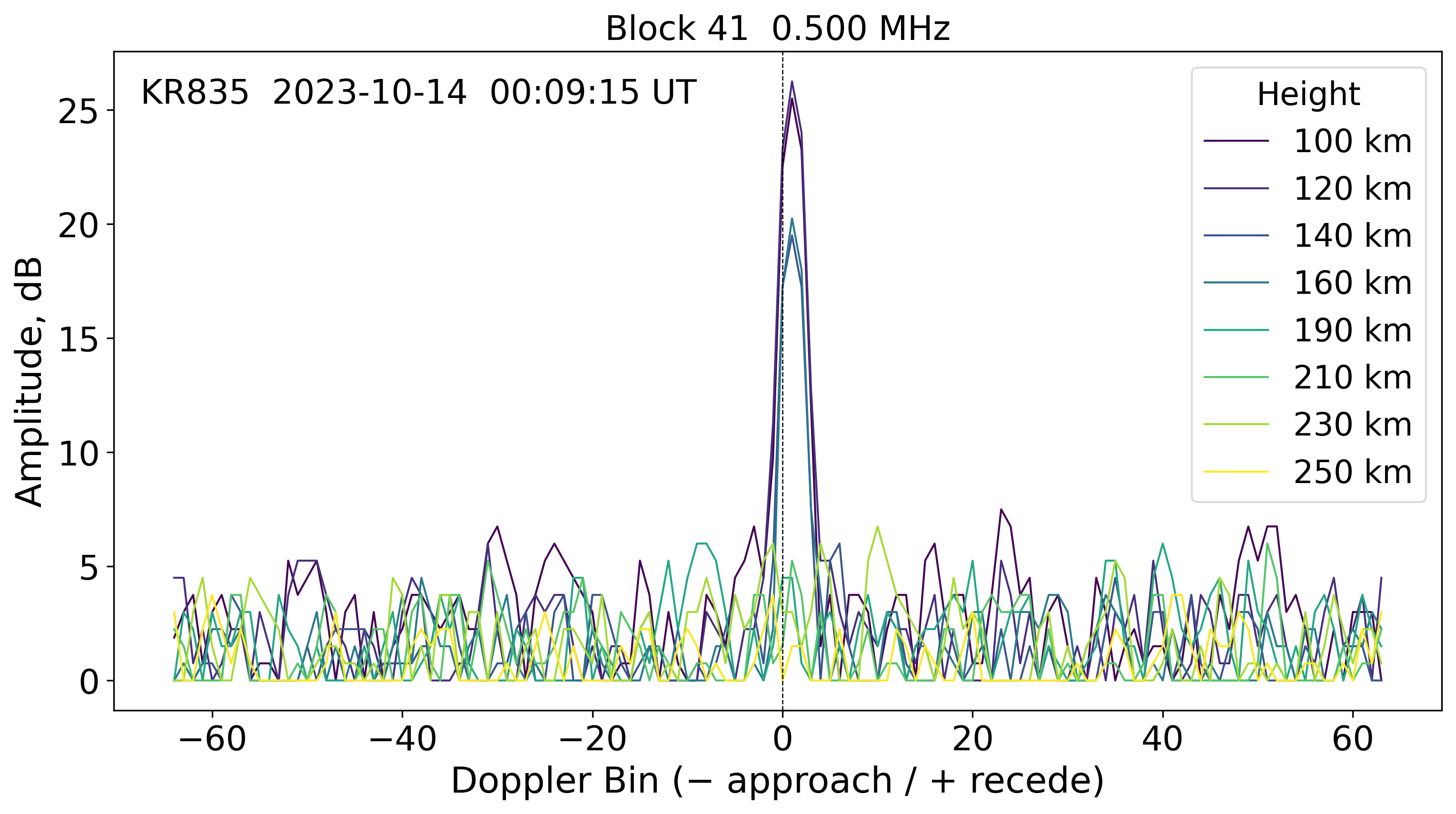
Related Files
examples/digisonde/sao_iso_dft_plots.pypynasonde/digisonde/parsers/sao.pypynasonde/digisonde/parsers/dft.pypynasonde/digisonde/digi_plots.py—SaoSummaryPlots.add_isodensity_contours(),SkySummaryPlots.plot_doppler_waterfall(),SkySummaryPlots.plot_doppler_spectra()