SAO — Scaled Ionogram Height Profiles and F2-Layer Diagnostics
End-to-End SAO Workflow
Load a full day of DPS4D .SAO files in parallel, extract
electron-density height profiles, and produce publication-ready
time–height and F2-layer diagnostic figures.
This page explains examples/digisonde/sao.py.
Data used: KR835 (Kirtland AFB) during the 14 October 2023 Great American Annular Eclipse.
Call Flow
SaoExtractor.load_SAO_files(...)scans the directory for.SAOfiles and parses them in parallel usingn_procsworkers.- For height profiles: request
func_name="height_profile"→ rows contain(datetime, th, pf, ed)per sounding. - For scaled parameters: request
func_name="scaled"→ rows contain(datetime, foF2, hmF2, …)summary values. SaoSummaryPlotsproduces time–height pcolormesh plots (add_TS) and dual-axis line plots (plot_TS) for scaled parameters.- Figures are saved to the docs assets tree for reuse.
Key Code
1) Load Height Profiles
import datetime as dt
import matplotlib.dates as mdates
from pynasonde.digisonde.parsers.sao import SaoExtractor
from pynasonde.digisonde.digi_plots import SaoSummaryPlots

date = dt.datetime(2023, 10, 14)

df = SaoExtractor.load_SAO_files(
    folders=["path/to/SKYWAVE_DPS4D_2023_10_14/"],
    func_name="height_profile",
    n_procs=8,
)
df.ed = df.ed / 1e6    # rescale to ×10⁶ cm⁻³ for colorbar clarity
2) Time–Height Electron Density Plot
sao_plot = SaoSummaryPlots(
    figsize=(6, 3),
    fig_title="KR835 / Height profiles during 14 Oct 2023 GAE",
    draw_local_time=False,
)
sao_plot.add_TS(
    df,
    zparam="ed",
    prange=[0, 1],
    zparam_lim=10,
    cbar_label=r"$N_e$, $\times 10^6$ /cc",
    plot_type="scatter",
    scatter_ms=20,
)
ax = sao_plot.axes
ax.set_xlim([date, date + dt.timedelta(1)])
ax.xaxis.set_major_locator(mdates.HourLocator(interval=6))
sao_plot.save("docs/examples/figures/stack_sao_ne.png")
sao_plot.close()
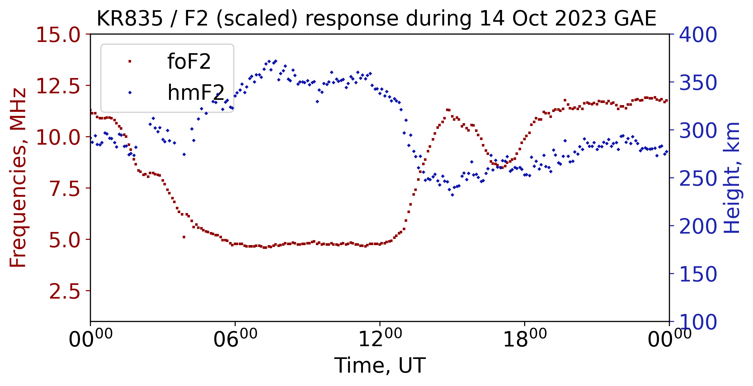
3) Load Scaled Parameters and Plot F2 Diagnostics
df_sc = SaoExtractor.load_SAO_files(
    folders=["path/to/SKYWAVE_DPS4D_2023_10_14/"],
    func_name="scaled",
    n_procs=8,
)

sao_plot = SaoSummaryPlots(
    figsize=(6, 3),
    fig_title="KR835 / F2 response during 14 Oct 2023 GAE",
    draw_local_time=False,
)
sao_plot.plot_TS(
    df_sc,
    right_yparams=["hmF2"],
    left_yparams=["foF2"],
    right_ylim=[100, 400],
    left_ylim=[1, 15],
)
ax = sao_plot.axes
ax.set_xlim([date, date + dt.timedelta(1)])
ax.xaxis.set_major_locator(mdates.HourLocator(interval=6))
sao_plot.save("docs/examples/figures/stack_sao_F2.png")
sao_plot.close()
Run
Output Figures

Related Files
examples/digisonde/sao.pypynasonde/digisonde/parsers/sao.pypynasonde/digisonde/digi_plots.py