Examples

Executable Workflows

Hands-on examples for loading ionosonde data, processing soundings, and producing publication-ready figures.

DIGISONDE Examples

DVL — Drift Velocity Stack Plot Load a full day of DPS4D .DVL files in parallel and produce a three-panel stacked drift velocity figure with a virtual-height overlay.
Open Example

SKY — Sky Map Visualization Parse DIGISONDE .SKY files, build single-panel polar sky maps colored by Doppler frequency, and combine multiple soundings into a multi-panel comparison figure.
Open Example

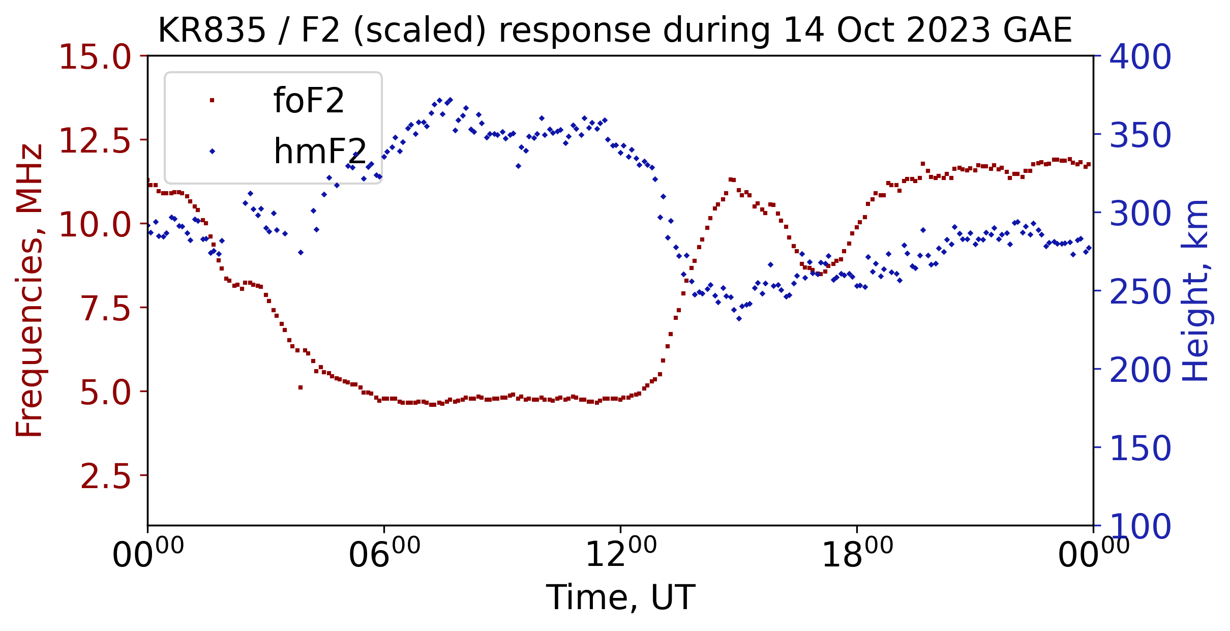
SAO — Height Profiles and F2 Diagnostics Extract electron-density height profiles and scaled F2-layer parameters from DPS4D .SAO files; produce time–height and dual-axis line plots.
Open Example

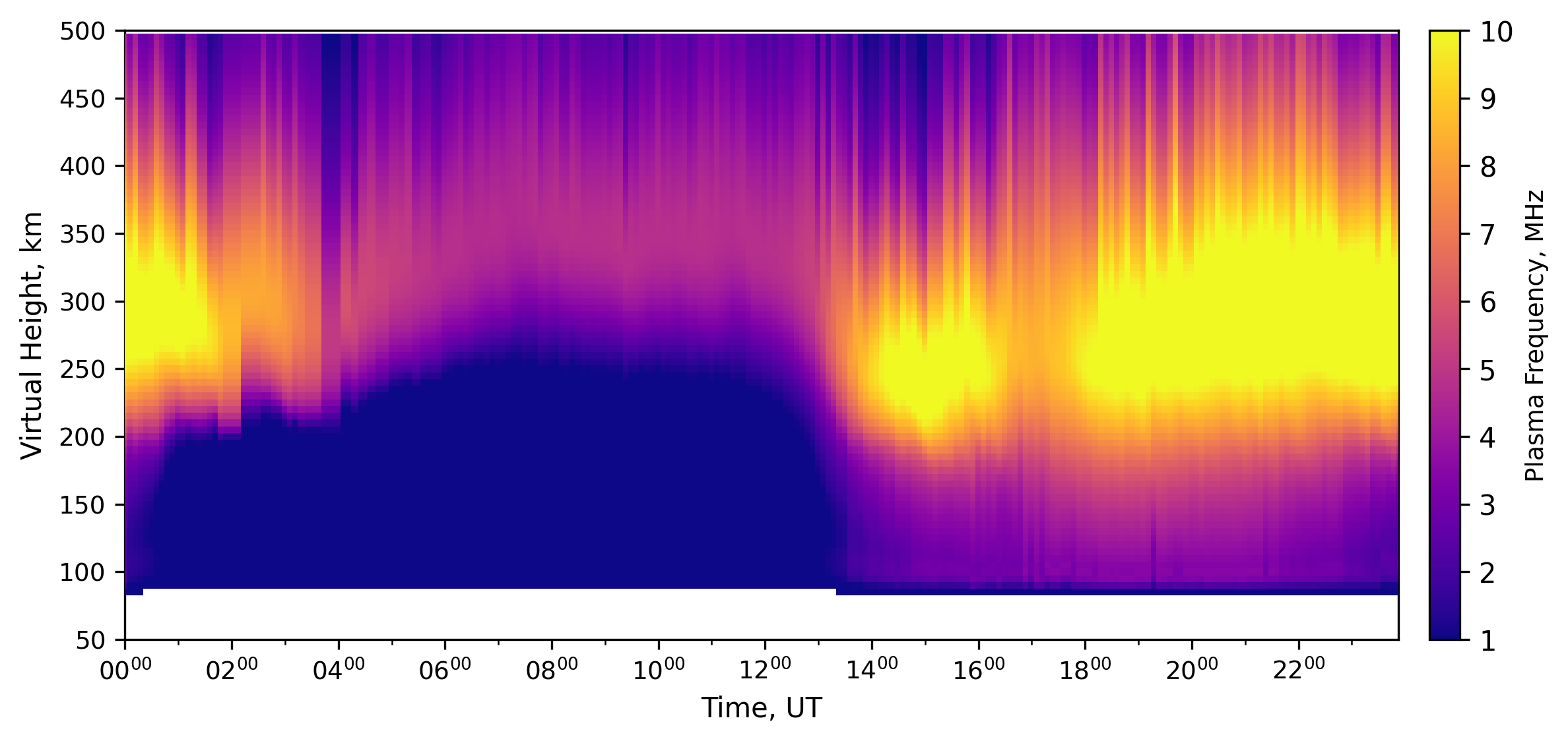
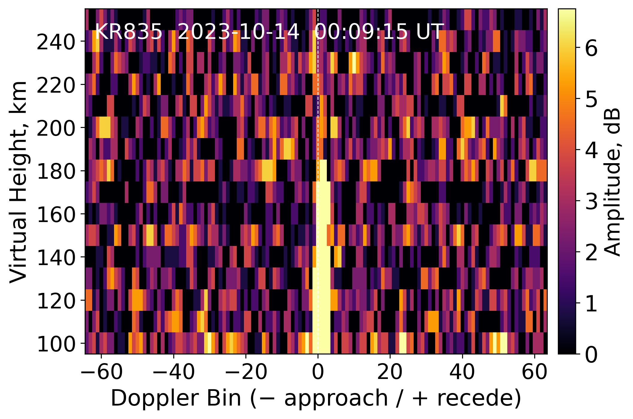
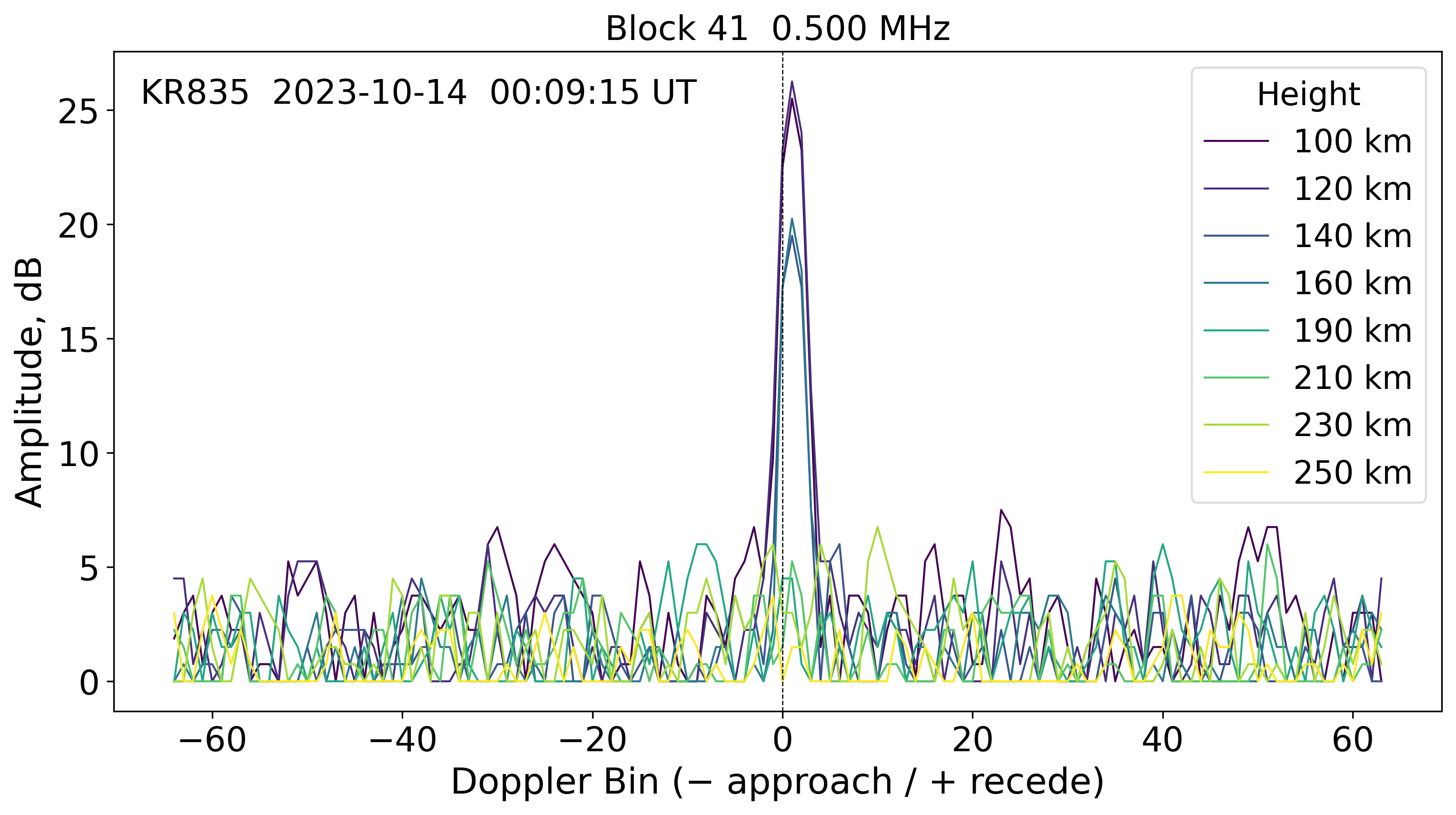
SAO + DFT — Isodensity Contours, Doppler Waterfall, and Spectra Build a daily isodensity contour from hundreds of .SAO files, then visualize the Doppler waterfall and per-height spectra from a single .DFT file.
Open Example

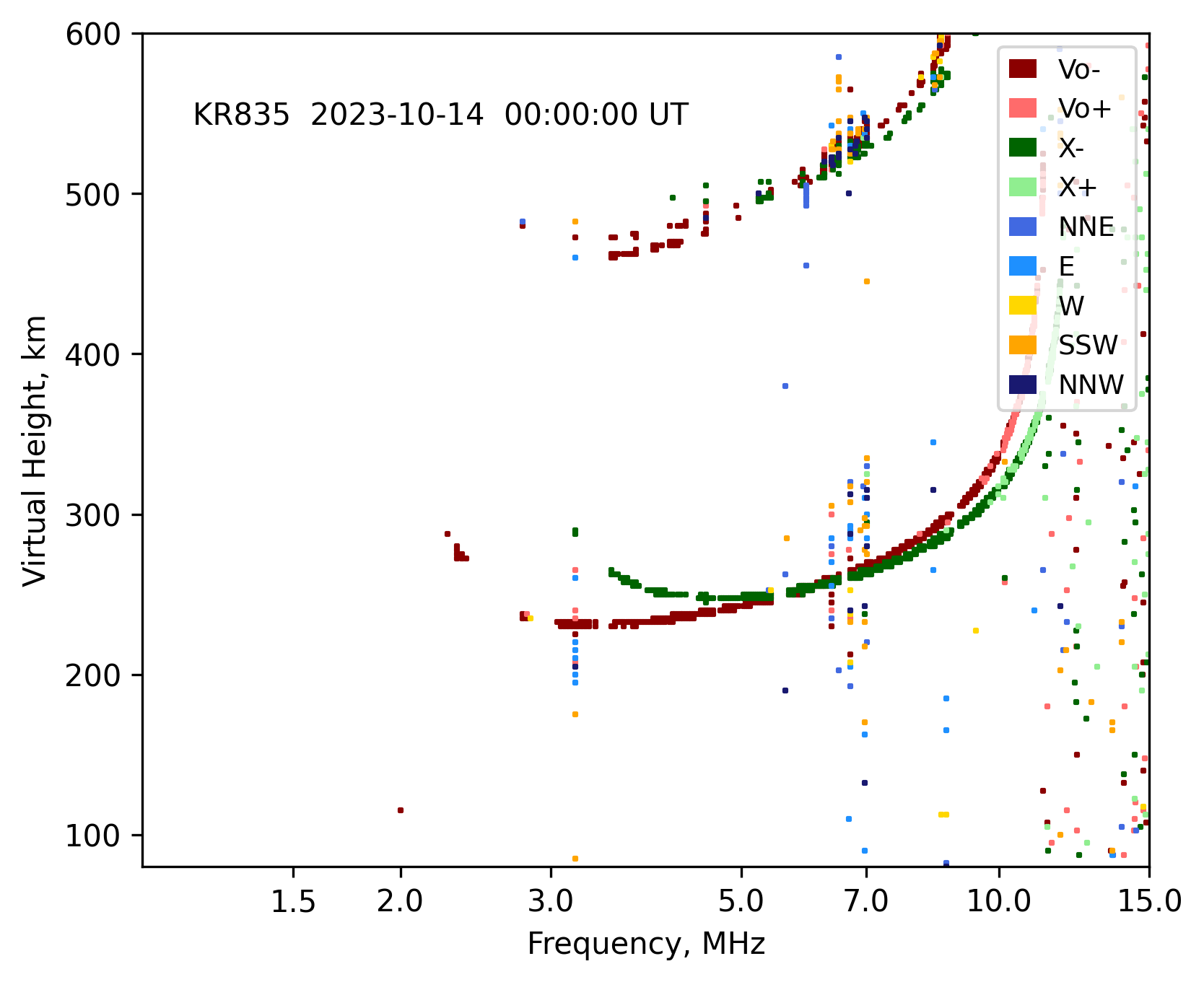
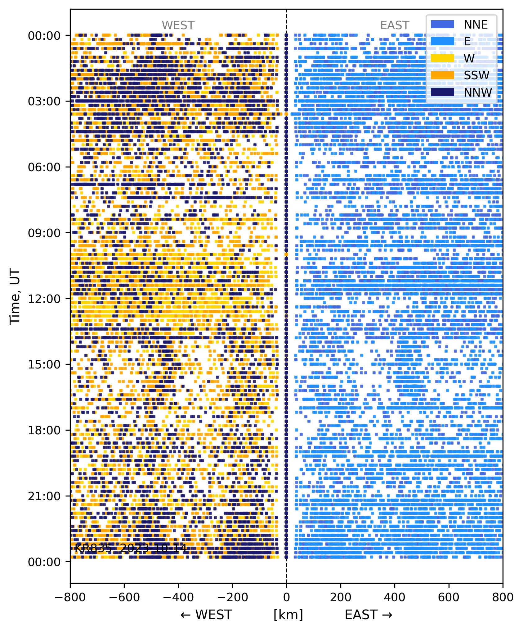
RSF — Direction-Coded Ionogram and Daily Directogram Parse raw DPS4D .RSF sounding files, render a direction-coded ionogram for a single record, and stack a full day into a directogram (time vs. ground distance).
Open Example

RSF — Parse and Inspect Raw Sounding File Low-level walkthrough: load a single .RSF file, parse all blocks and frequency groups into structured Python dataclasses, and inspect headers programmatically.
Open Example

VIPIR Examples

RIQ — Echo Extraction (PL407) Extract Dynasonde 7-parameter echoes (height, amplitude, V*, EP, PP, XL, YL) from a VIPIR PL407 .RIQ file and inspect the resulting echo cloud.
Open Example

RIQ — Echo Extraction (WI937) Full 8-receiver echo extraction from a WI937 .RIQ file, including direction cosines (XL, YL), EP wavefront residual, and polarization. Demonstrates SNR thresholding and height filtering.
Open Example

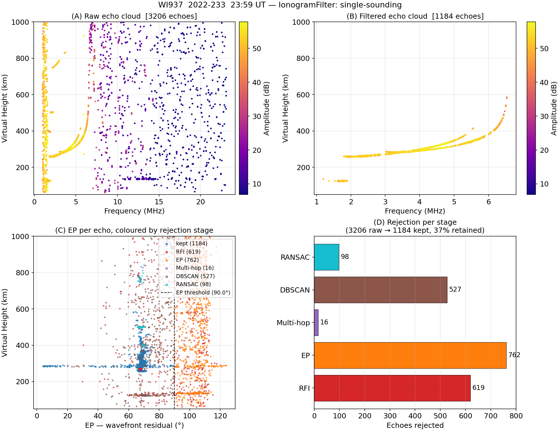
RIQ — Ionogram Filter (single & multi-sounding) Apply the six-stage IonogramFilter (RFI blanking, EP, multi-hop, DBSCAN, RANSAC, temporal coherence) to reject noise from a VIPIR echo cloud. Covers WI937, PL407, and multi-sounding configurations.
Open Example

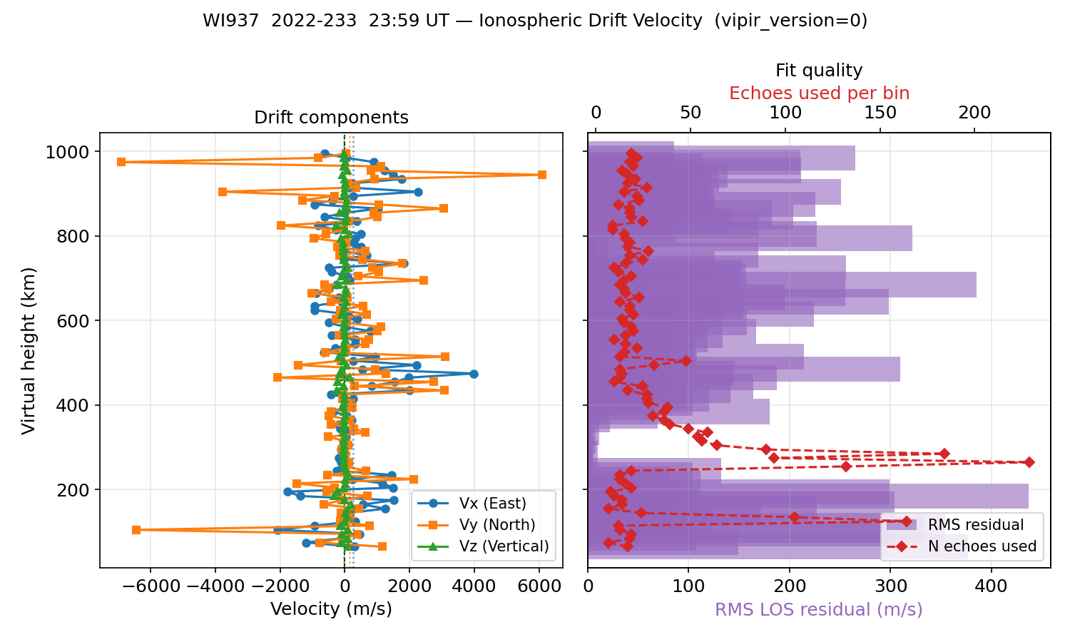
RIQ — Drift Velocity (WI937) Estimate the 3-D ionospheric drift vector [Vx, Vy, Vz] from line-of-sight velocities using height-binned weighted least-squares with iterative sigma-clipping. Includes whole-sounding and height-resolved fits.
Open Example

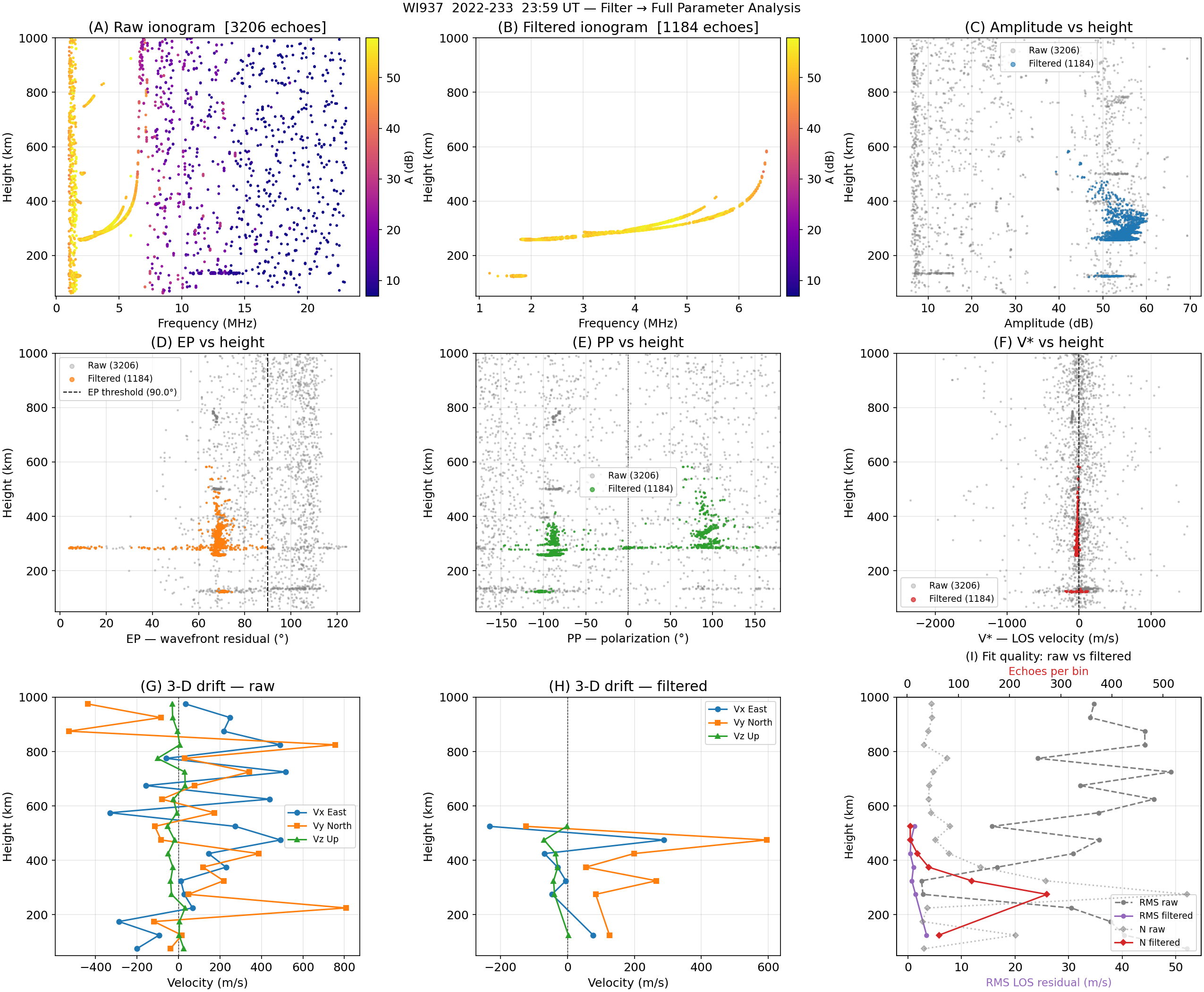
RIQ — Full Parameter Analysis (WI937) End-to-end workflow: filter a WI937 sounding, then compare amplitude, EP, PP, V*, and 3-D drift velocity between raw and filtered echo clouds in a 3×3 diagnostic figure.
Open Example

RIQ — Ionogram from Raw Capture Read a VIPIR .RIQ file, clean the ionogram with the adaptive gain filter, and plot O/X-mode power on a frequency–virtual-height canvas.
Open Example

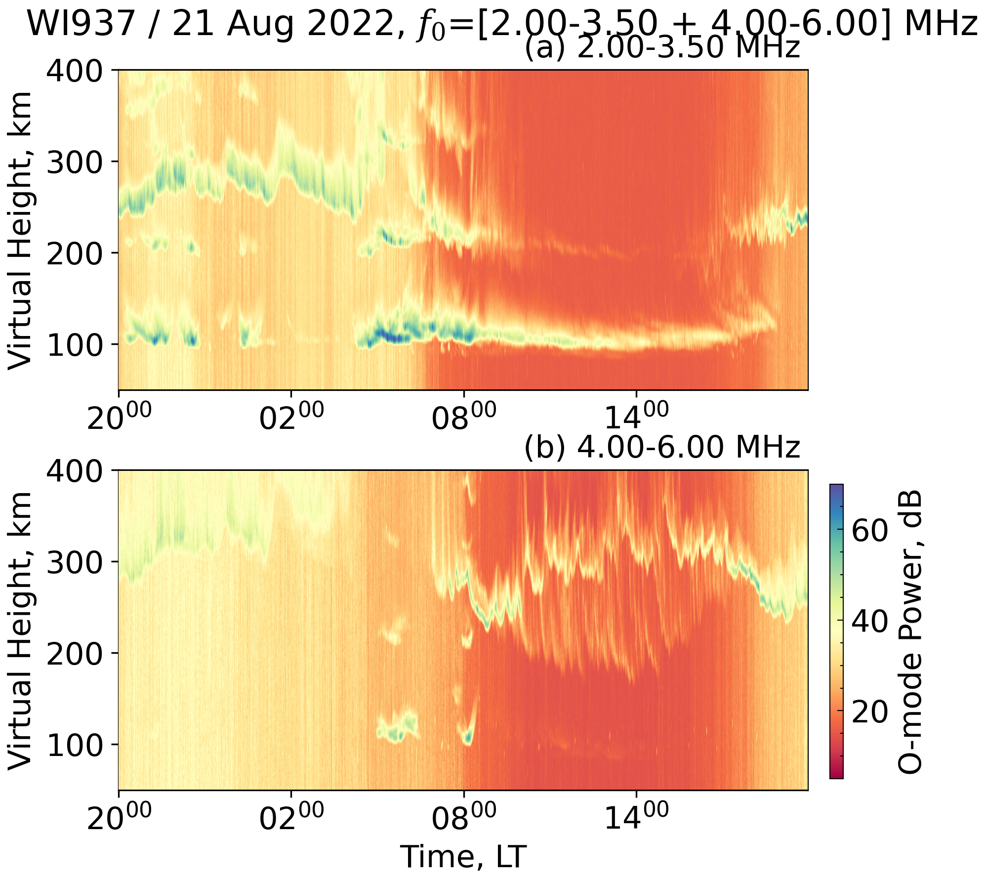
NGI — Frequency–Time Interval (FTI) Plot Load a day of VIPIR NGI ionogram cubes in parallel, flatten per-band power grids into a long-form dataframe, and produce O-mode FTI stacked panels.
Open Example

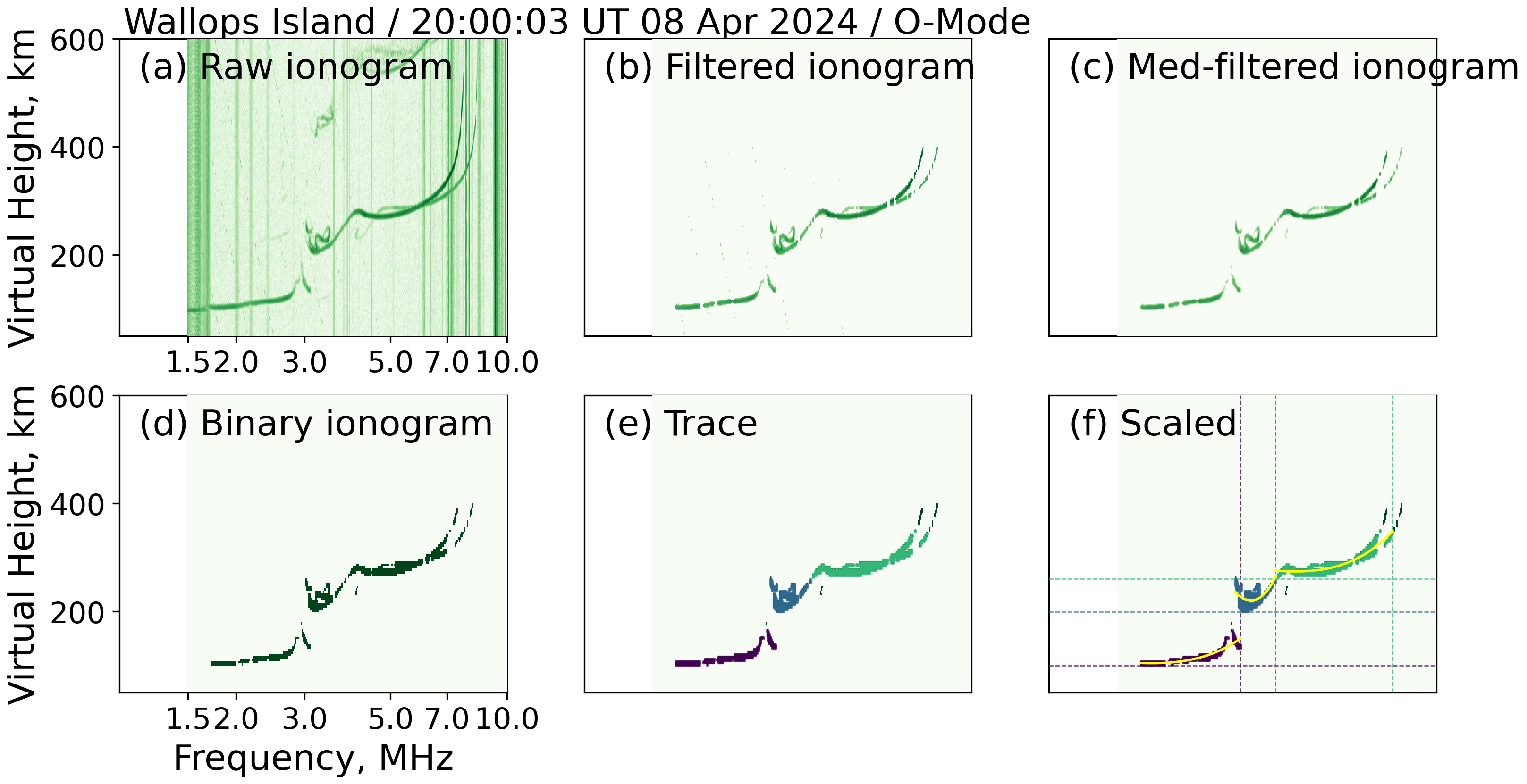
NGI — AutoScaler Sanity-Check Figures Stage a day of NGI files, run the full autoscaling pipeline (median filter → image segmentation → Otsu + DBSCAN binary traces), and emit a QA sanity-check figure.
Open Example

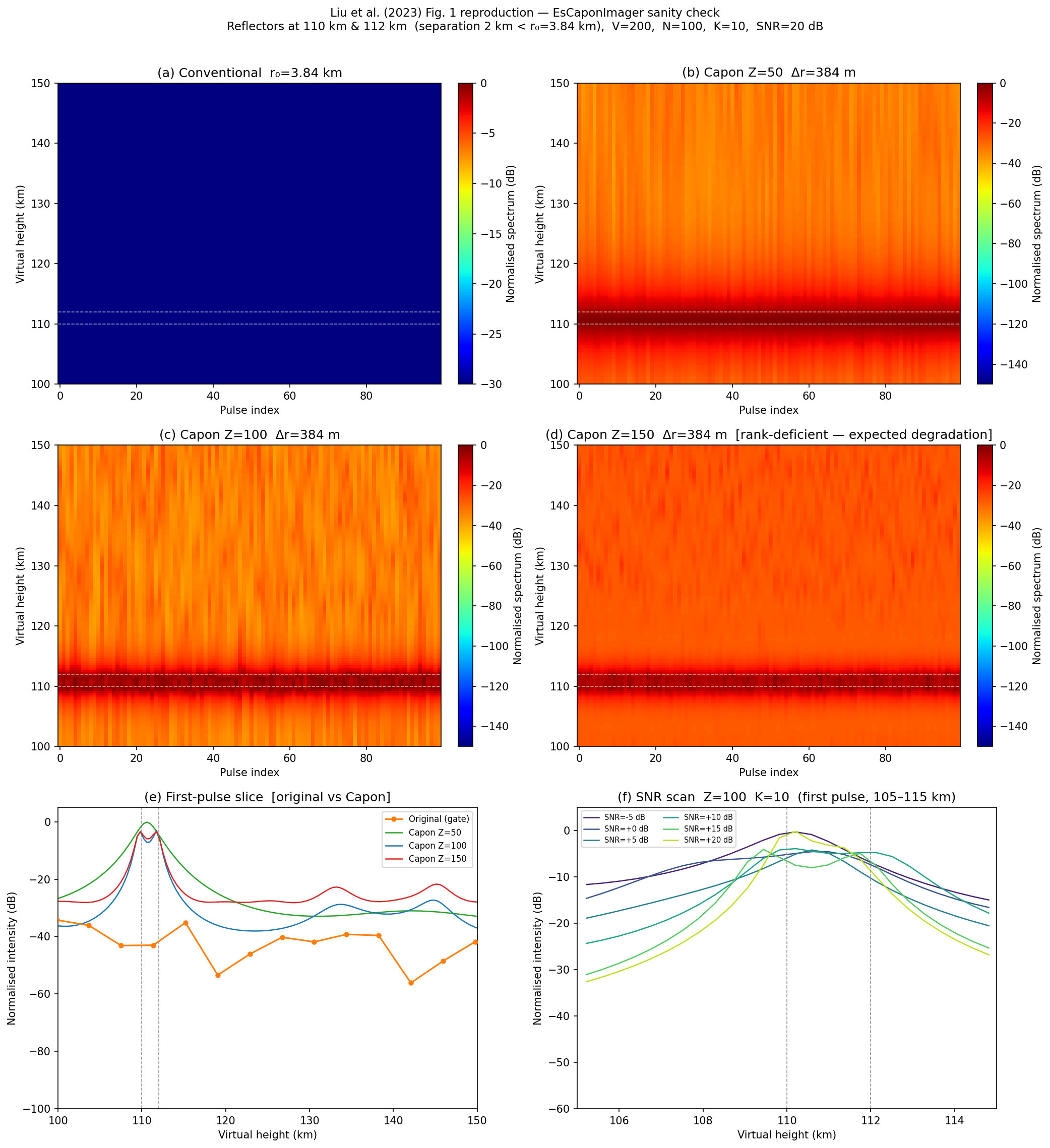
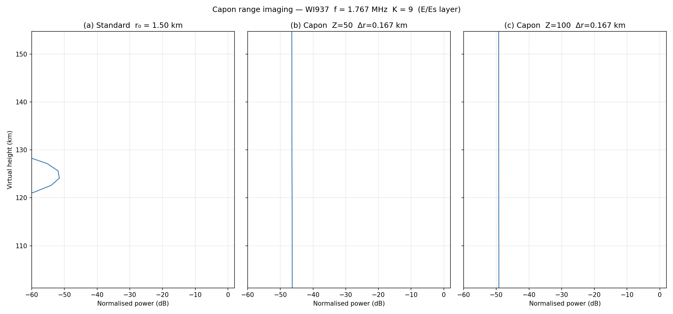
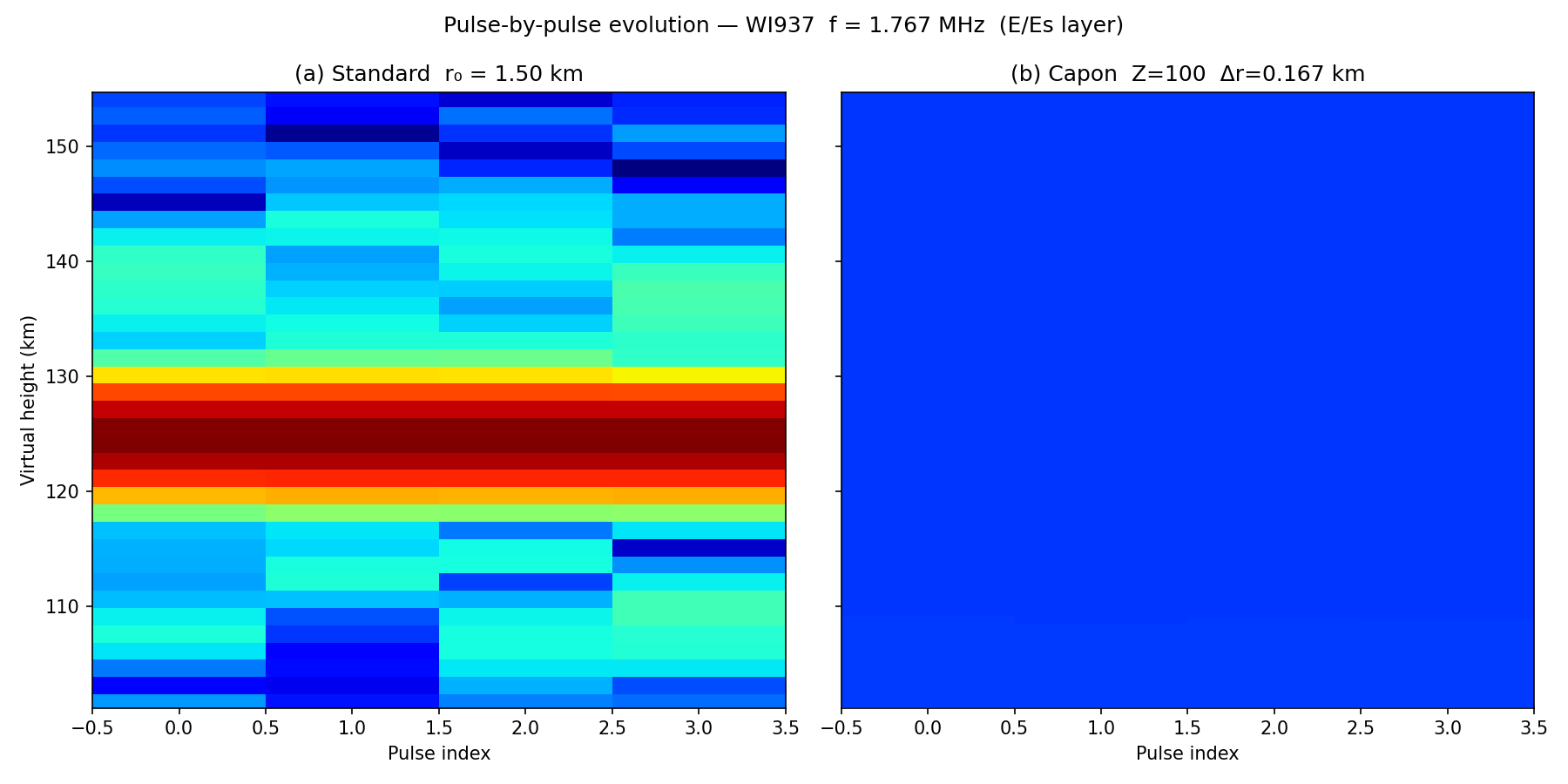
Analysis — Es Layer Imaging (Sanity Check) Reproduce Liu et al. (2023) Fig. 1: synthetic two-layer benchmark with Z=50/100/150 subbands, confirming the Capon imager resolves a 2 km layer separation invisible to conventional ranging.
Open Example

Analysis — Es Layer Imaging (Single File) Load a VIPIR RIQ file and run EsCaponImager to produce a high-resolution pseudospectrum with 10× finer range bins (150 m from a 1.499 km gate).
Open Example

Analysis — Es Layer Imaging (Multi-File A+B+C) Combine 8 VIPIR files (4 pulses × 8 Rx each) via RiqAggregator: coherent Rx beamforming (+9 dB) then incoherent pulse and file averaging (÷32 variance) for ~24 dB total SNR improvement.
Open Example

Figure Gallery