Es Layer Imaging — High-Resolution Capon Analysis
Sporadic-E Layer Imaging via Capon Cross-Spectrum Analysis
Achieve up to 10× finer range resolution from pulse-compressed RIQ gate data using the minimum-variance Capon estimator (Liu et al. 2023). Three complementary examples: algorithm validation, single-file imaging, and multi-file A+B+C aggregation.
This page covers three scripts:
| Script | What it demonstrates |
|---|---|
examples/vipir/analysis/es_imaging_sanity_check.py |
Reproduce Liu et al. (2023) Fig. 1 — synthetic two-layer validation |
examples/vipir/analysis/es_imaging_example.py |
Single RIQ file imaging with EsCaponImager |
examples/vipir/analysis/es_aggregator_example.py |
Multi-file A+B+C combining with RiqAggregator |
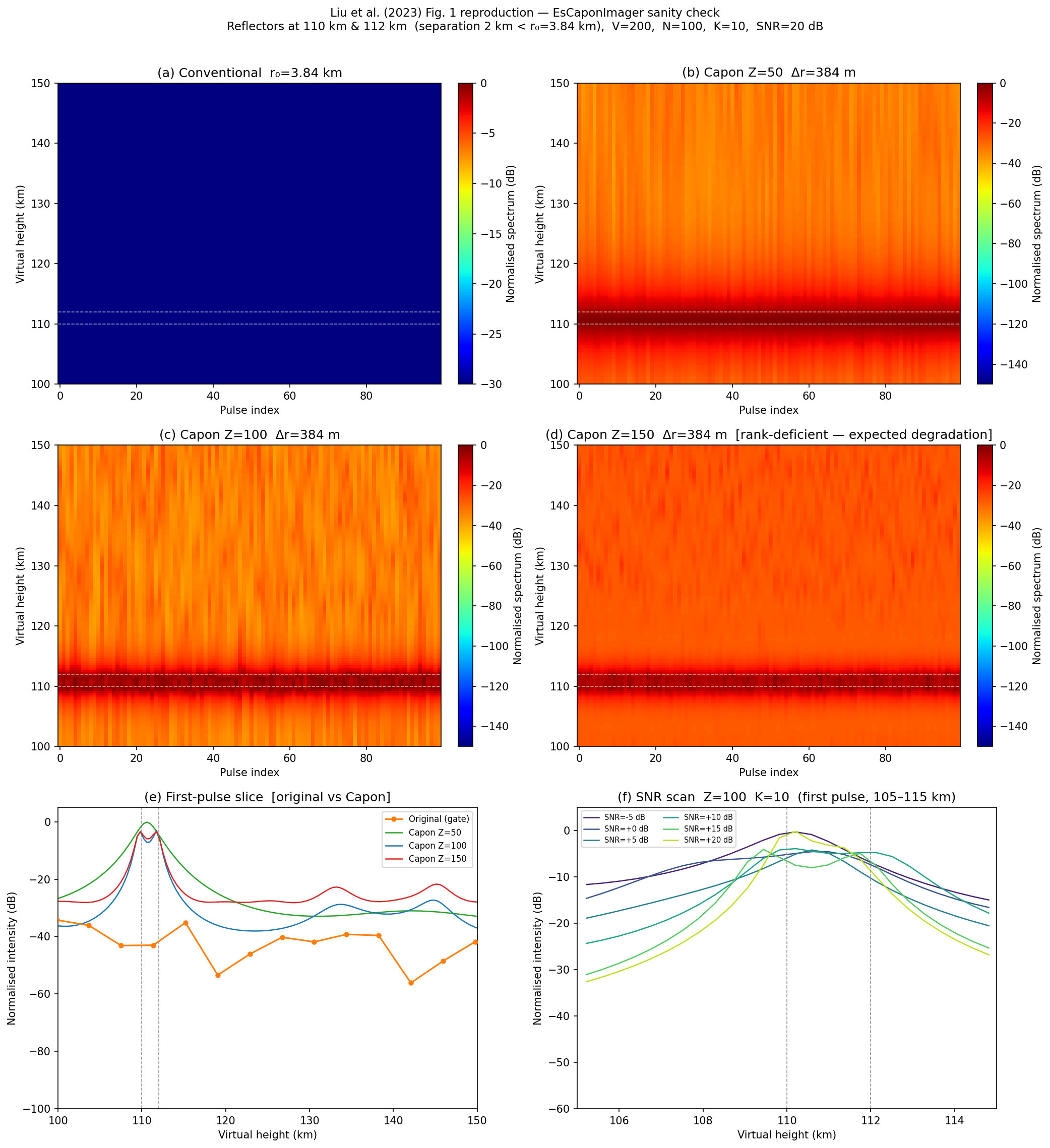
1 — Algorithm Sanity Check (Liu et al. Fig. 1 reproduction)
es_imaging_sanity_check.py validates the EsCaponImager implementation against
the synthetic two-layer benchmark from the paper.
Synthetic data construction
Two point scatterers are placed at D₁ = 110 km and D₂ = 112 km (2 km
separation — below the native gate resolution). Their spectral bins are:
The noiseless cross-power spectrum is:
m = np.arange(V)  # V = 200 spectral bins
G_ss = np.exp(1j * 2 * np.pi * Q1 * m / V) + np.exp(1j * 2 * np.pi * Q2 * m / V)
R_ss = np.fft.ifft(G_ss)  # range profile — one "pulse"
Gaussian noise is added to give a target SNR, then N=256 independent noisy pulses are generated.
Six-panel figure
| Panel | Z (subbands) | Observation |
|---|---|---|
| (a) Conventional (Z=1) | 1 | Single broad peak — cannot resolve 2 km |
| (b) Z=50 | 50 | Improved but still one peak (resolution limit) |
| (c) Z=100 | 100 | Two peaks resolved at ≈110 and ≈112 km |
| (d) Z=150 | 150 | Rank-deficient (Z > (V+1)/2=100), degraded |
| (e) First-pulse vs 256-pulse average | 100 | SNR improvement from pulse averaging |
| (f) SNR scan | 100 | Peak separation score vs input SNR |
Key result
With Z=100, K=10, V=200, the two layers are recovered at 109.82 km and
111.74 km (true: 110 and 112 km) — within 0.3 km of truth.
from pynasonde.vipir.analysis import EsCaponImager
import numpy as np

V, N, K = 200, 256, 10
r0 = 3.84        # km — WISS native gate
D1, D2 = 110.0, 112.0

Q1, Q2 = D1 / r0, D2 / r0
m = np.arange(V)
G_ss = np.exp(1j*2*np.pi*Q1*m/V) + np.exp(1j*2*np.pi*Q2*m/V)
R_ss = np.fft.ifft(G_ss)

# Add noise and stack N pulses
rng = np.random.default_rng(42)
noise_std = 10 ** (-20 / 20)   # 20 dB SNR
cube = (R_ss[None, :] + noise_std * (rng.standard_normal((N, V))
        + 1j * rng.standard_normal((N, V))) / np.sqrt(2))

imager = EsCaponImager(n_subbands=100, resolution_factor=10,
                       gate_spacing_km=r0, gate_start_km=0.0)
result = imager.fit(cube)
Run
cd /home/chakras4/Research/CodeBase/pynasonde
python examples/vipir/analysis/es_imaging_sanity_check.py
Output figure
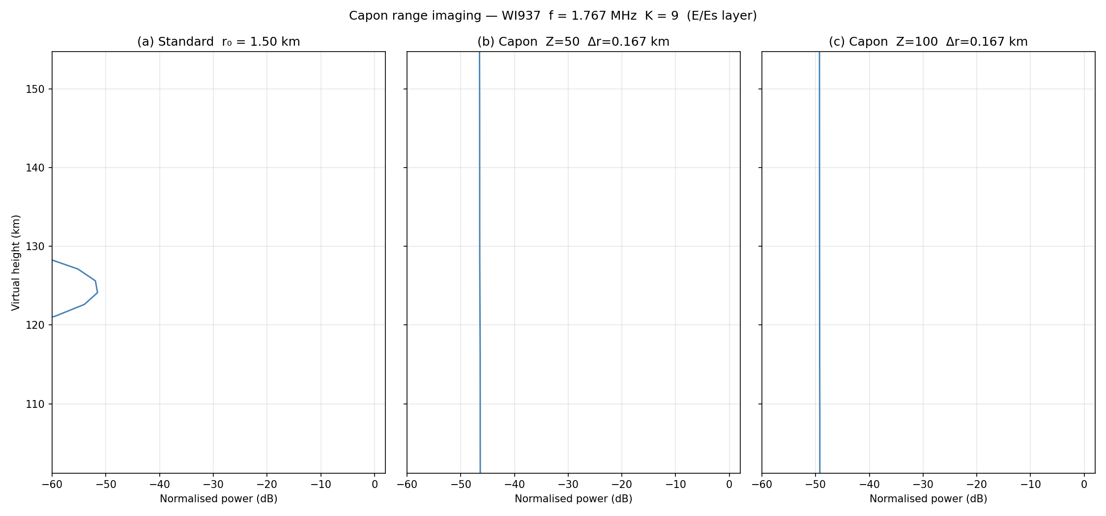
2 — Single-File Imaging (EsCaponImager)
es_imaging_example.py shows the end-to-end workflow for a real VIPIR RIQ file.
Call flow
RiqDataset.create_from_file(fname)
    └─ pulsets[freq_idx]
           └─ iq_cube  (pulse_count, gate_count, rx_count)
                  │
           EsCaponImager.fit(iq_cube)
                  └─► EsImagingResult
                            ├─ .plot()         # RTI or profile
                            └─ .to_dataframe() # height_km, power_db
Step-by-step
from pynasonde.vipir.riq.parsers.read_riq import RiqDataset
from pynasonde.vipir.analysis import EsCaponImager

# 1. Load RIQ file and extract IQ cube at target frequency
riq = RiqDataset.create_from_file("path/to/file.RIQ")
pulset = riq.pulsets[0]                    # first frequency step
iq_cube = pulset.iq_cube()                 # (pulse_count, gate_count, rx_count)

# 2. Configure imager (VIPIR parameters)
imager = EsCaponImager(
    n_subbands=100,
    resolution_factor=10,
    gate_spacing_km=1.499,      # VIPIR r₀ ≈ c × 10 µs / 2
    gate_start_km=90.0,
    rx_index=0,                 # single channel
    coherent_integrations=1,    # per-pulse imaging
)

# 3. Image
result = imager.fit(iq_cube)
print(result.summary())
# EsImagingResult: snapshots=4  Z=100  K=10  r₀=1.499 km → Δr=0.150 km
# height=90.0–1527.9 km

# 4. Plot
result.plot(snapshot=0)         # single-pulse profile
result.plot()                   # RTI across all pulses
Output figure
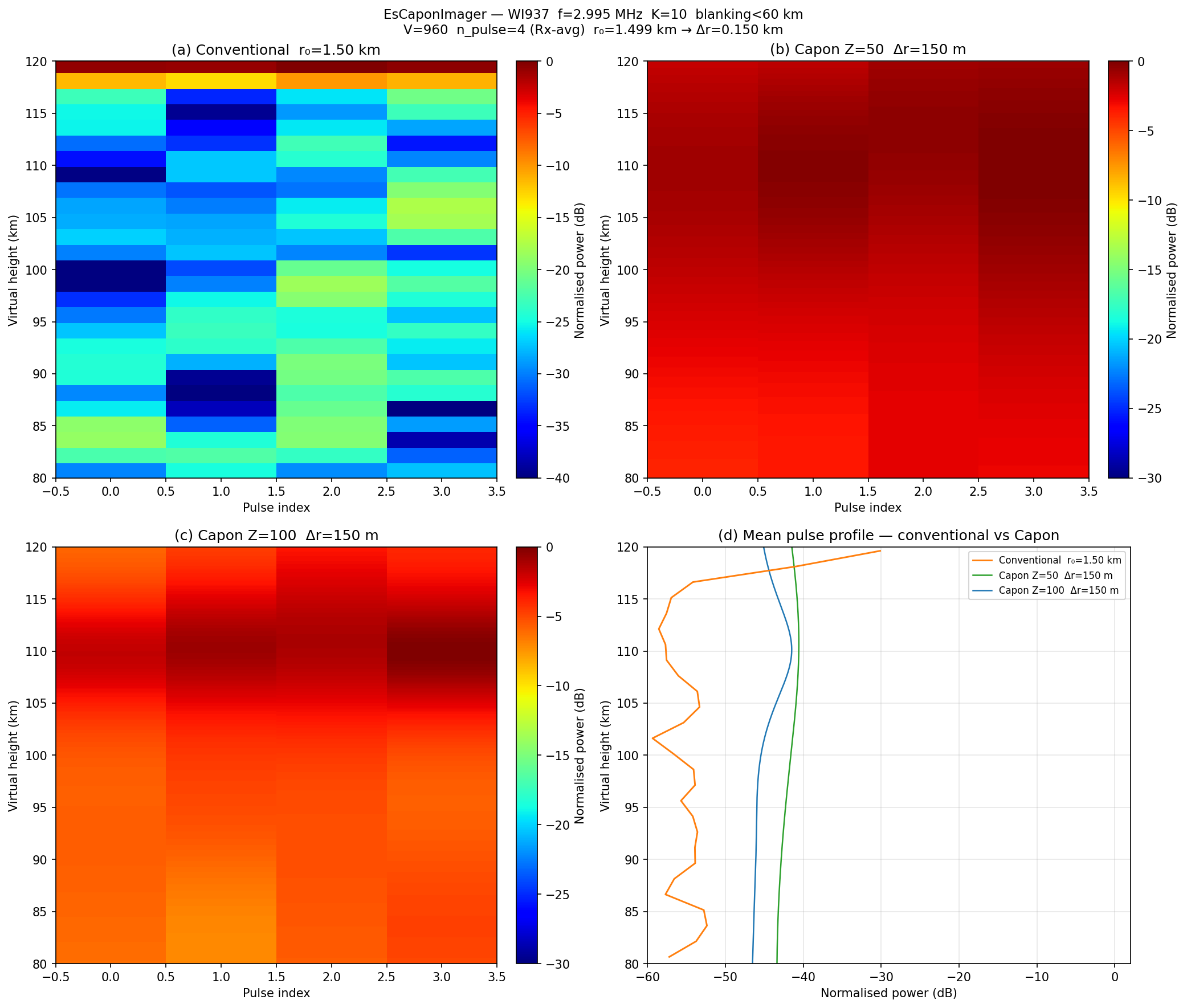
3 — Aggregator Example: Single-File Sanity + 20-File Time-Series
es_aggregator_example.py has two sections:
Figure 1 — single-file sanity check (4 panels, first matched file):
Loads the pulset closest to FREQ_TARGET_KHZ = 3000.0 kHz, averages the 8 Rx
channels per pulse → (n_pulse, n_gate) cube, applies gate blanking below 60 km,
then runs EsCaponImager with Z=50 and Z=100.
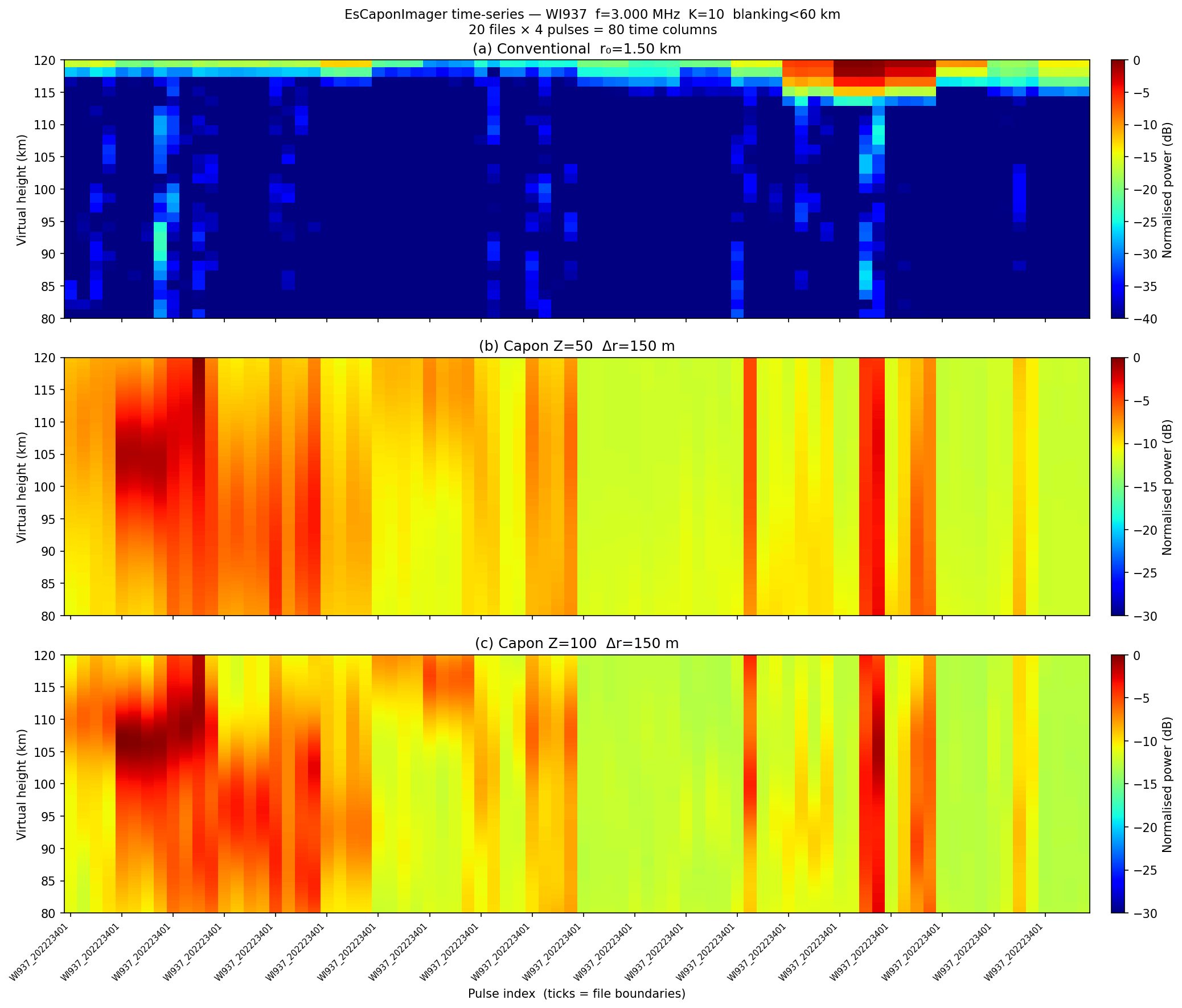
Figure 2 — 20-file time-series RTI (3 panels, up to MAX_FILES = 20 files):
Processes files in parallel using ThreadPoolExecutor. Each file contributes
n_pulse = 4 time columns (one per pulse), giving up to 80 columns total.
Key design decisions (Liu et al. 2023)
All snapshots fed to the Capon covariance must be at the same carrier frequency. Different frequencies see different ionospheric reflectors (Es only reflects below foEs); mixing them corrupts the covariance matrix.
The 8 Rx channels are averaged per pulse (not stacked as independent snapshots)
to produce a clean (n_pulse, n_gate) 2-D cube. Gate blanking (blank_min_km=60)
zeros the leading gates before the Capon covariance so the direct-wave clutter
peak does not dominate R_f.
Call flow
_load_cube(riq_path, freq_khz=3000.0)
    └─ find closest pulset
    └─ for each PCT: average 8 Rx → (n_gate,) profile
    └─ stack → (n_pulse, n_gate)

_blank(cube, gate_blank)          # zero gates below 60 km

EsCaponImager.fit(cube)           # (n_pulse, K*V) pseudospectrum_db
    └─ per pulse: FFT → _covariance(G_ss) → _capon(R_inv, A)
Parallel time-series
from concurrent.futures import ThreadPoolExecutor, as_completed

def _process_file(src):
    cube, r0, g0, _ = _load_cube(src, FREQ_TARGET_KHZ, VIPIR_VERSION_IDX)
    blk   = _blank(cube, max(0, int((BLANK_MIN_KM - g0) / r0)))
    r50   = _run_capon(blk, Z=50,  K=10, gate_start_km=g0, gate_spacing_km=r0)
    r100  = _run_capon(blk, Z=100, K=10, gate_start_km=g0, gate_spacing_km=r0)
    return dict(conv=..., cap50=r50.pseudospectrum_db, cap100=r100.pseudospectrum_db, ...)

with ThreadPoolExecutor() as executor:
    futures = {executor.submit(_process_file, src): i
               for i, src in enumerate(ts_paths)}
    for future in as_completed(futures):
        ordered[futures[future]] = future.result()
numpy releases the GIL during np.fft.fft, np.linalg.inv, and np.einsum,
so multiple files run Capon concurrently on separate OS threads.
Output figures
Run all examples
cd /home/chakras4/Research/CodeBase/pynasonde

# Algorithm validation (no real data needed)
python examples/vipir/analysis/es_imaging_sanity_check.py

# Single-file imaging
python examples/vipir/analysis/es_imaging_example.py

# Multi-file aggregation
python examples/vipir/analysis/es_aggregator_example.py
Related files
pynasonde/vipir/analysis/es_imaging/capon.py—EsCaponImager,EsImagingResultpynasonde/vipir/analysis/es_imaging/aggregator.py—RiqAggregatorpynasonde/vipir/analysis/es_imaging/__init__.py— package re-exportsexamples/vipir/analysis/es_imaging_sanity_check.pyexamples/vipir/analysis/es_imaging_example.pyexamples/vipir/analysis/es_aggregator_example.py
References
Liu, T., Yang, G., & Jiang, C. (2023). High-resolution sporadic E layer observation based on ionosonde using a cross-spectrum analysis imaging technique. Space Weather, 21, e2022SW003195. https://doi.org/10.1029/2022SW003195